Writing Reports with R Markdown
Overview
Teaching: 90 min
Exercises: 30 minQuestions
How can I make reproducible reports using R Markdown?
How do I format text using Markdown?
Objectives
To create a report in R Markdown that combines text, code, and figures.
To use Markdown to format our report.
To understand how to use R code chunks to include or hide code, figures, and messages.
To be aware of the various report formats that can be rendered using R Markdown.
Contents
- What is R Markdown and why use it?
- Creating a reports directory
- Creating an R Markdown file
- Basic components of R Markdown
- Starting the report
- Formatting
- Knitting to PDF
Recall that our goal is to generate a report which analyses how environmental conditions change microbial communities in Lake Ontario.
Discussion
How do you usually share data analyses with your collaborators? Add your usual workflow to the Etherpad.
What is R Markdown and why use it?
In R Markdown, you can incorporate ordinary text (ex. experimental methods, analysis and discussion of results) alongside code and figures! (Some people write entire manuscripts in R Markdown - if you’re curious, talk to the Schmidt Lab!) This is useful for writing reproducible reports and publications, sharing work with collaborators, writing up homework, and keeping a bioinformatics notebook. Because the code is embedded in the document, the tables and figures are reproducible. Anyone can run the code and get the same results. If you find an error or want to add more to the report, you can just re-run the document and you’ll have updated tables and figures! This concept of combining text and code is called “literate programming”. To do this we use R Markdown, which combines Markdown (renders plain text) with R. You can output an html, PDF, or Word document that you can share with others. In fact, this webpage is an example of a rendered R markdown file!
(If you are familiar with Jupyter notebooks in the Python programming environment, R Markdown is R’s equivalent of a Jupyter notebook.)
Other Options for Literate Programming
There are many options for combining code and prose. If you are familiar with Jupyter notebooks in the Python programming environment, R Markdown is R’s equivalent of a Jupyter notebook. The company which manages RStudio, Posit, has also invested considerable energy in a new document type “Quarto”, which they encourage users to adopt as it does not rely on an R install. There are many similarities between Quarto and RMarkdown, but the community of Quarto users (and history of troubleshooting support) is still smaller. Maybe someday soon, we will be teaching Quarto documents instead!
Creating a reports directory
To get started, let’s use the Unix Shell to create a directory within ontario-report called reports where we will write our reports.
First, open the Unix Shell and cd to ontario-report:
pwd
mkdir reports
/home/USERNAME/Desktop/ontario-report/reports/
Note that there is an option to use the terminal from R Studio (tab next to Console), but on Windows computers this terminal might not be a Unix Shell.
Creating an R Markdown file
Now that we have a better understanding of what we can use R Markdown files for, let’s start writing a report!
To create an R Markdown file:
- Open RStudio
- Go to File → New File → R Markdown
- Give your document a title, something like “A Report on Lake Ontario’s Microbes” (Note: this is not the same as the file name - it’s just a title that will appear at the top of your report)
- Keep the default output format as HTML.
- R Markdown files always end in
.Rmd
R Markdown Outputs
The default output for an R Markdown report is HTML, but you can also use R Markdown to output other report formats. For example, you can generate PDF reports using R Markdown, but you must install some form of LaTeX to do this.
Basic components of R Markdown
Header
The first part is a header at the top of the file between the lines of ---. This contains instructions for R to specify the type of document to be created and options to choose (ex., title, author, date). These are in the form of key-value pairs (key: value; YAML).
Here’s an example:
---
title: 'Writing Reports with R Markdown'
author: "Augustus Pendleton"
date: "01/14/2025"
output: html_document
---
Code chunks
The next section is a code chunk, or embedded R code, that sets up options for all code chunks. Here is the default when you create a new R Markdown file:
```{r setup, include=FALSE}
knitr::opts_chunk$set(echo = TRUE)
```
All code chunks have this format:
```{r}
# Your code here
```
All of the code is enclosed in 3 back ticks and the {r} part indicates that it’s a chunk of R code.
You can also include other information within the curly brackets to indicate different information about that code chunk.
For instance, the first code block is named “setup”, and include=FALSE prevents code and results from showing up in the output file.
Inside the code chunk, you can put any R code that you want to run, and you can have as many code chunks as you want in your file.
As we mentioned above, in the first code chunk you set options for the entire file.
echo = TRUE means that you want your code to be shown in the output file. If you change this to echo = FALSE, then the code will be hidden and only the output of the code chunks will be seen in the output file.
There are also many other options that you can change, but we won’t go into those details in this workshop.
Text
Finally, you can include text in your R Markdown file. This is any text or explanation you want to include, and it’s formatted with Markdown. We’ll learn more about Markdown formatting soon!
Starting the report
Let’s return to the new R Markdown file you created and delete everything below the setup code chunk. (That stuff is just examples and reminders of how to use R Markdown.)
Next, let’s save our R markdown file to the reports directory.
You can do this by clicking the save icon in the top left or using control + s (command + s on a Mac). Make sure to end the file with a “.Rmd” file extension.
There’s one other thing that we need to do before we get started with our report.
To render our documents into html format, we can “knit” them in R Studio.
Usually, R Markdown renders documents from the directory where the document is saved (the location of the .Rmd file), but we want it to render from the main project directory where our .Rproj file is.
This is because that’s where all of our relative paths are from and it’s good practice to have all of your relative paths from the main project directory.
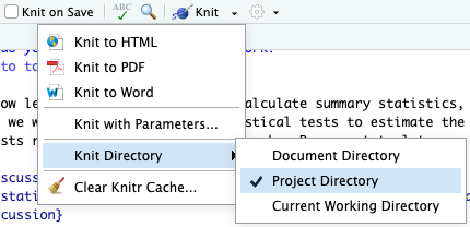
To change this default, click on the down arrow next to the “Knit” button at the top left of R Studio, go to “Knit Directory” and click “Project Directory”.
Now it will assume all of your relative paths for reading and writing files are from the ontario-report directory, rather than the reports directory.
Now that we have that set up, let’s start on the report!
We’re going to use the code you generated yesterday to plot cell abundance and temperature to include in the report. Recall that we needed a couple R packages to generate these plots. We can create a new code chunk to load the needed packages. You could also include this in the previous setup chunk, it’s up to your personal preference.
```{r packages}
library(tidyverse)
```
Now, in a real report this is when we would type out the background and purpose of our analysis to provide context to our readers. However, since writing is not a focus of this workshop we will avoid lengthy prose and stick to short descriptions. You can copy the following text into your own report below the package code chunk.
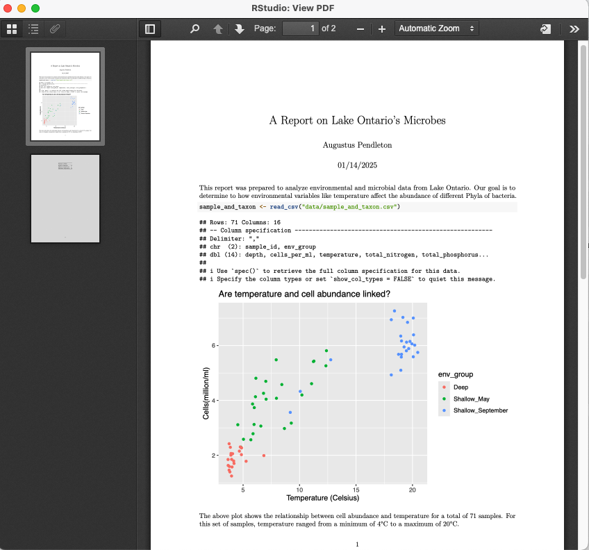
This report was prepared to analyze environmental and microbial data from Lake Ontario. Our goal is to determine to how environmental variables like temperature affect the abundance of different Phyla of bacteria.
Now, since we want to show our results comparing cell abundance and temperature, we need to read in this data so we can regenerate our plot. We will add another code chunk to prepare the data.
```{r data}
sample_and_taxon <- read_csv("data/sample_and_taxon.csv")
```
Now that we have the data, we need to produce the plot. Let’s create it!
```{r cell_vs_temp}
ggplot(data = sample_and_taxon) +
  aes(x = temperature, y = cells_per_ml/1000000, color=env_group) +
  geom_point() +
  labs(x = "Temperature (Celsius)", y = "Cells(million/ml)",
       title= "Are temperature and cell abundance linked?")
```
Now we can knit our document to see how our report looks! Use the knit button in the top left of the screen.
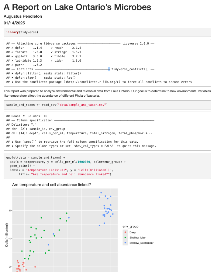
It’s looking pretty good, but there seem to be a few extra bits that we don’t need in the report. For example, the report shows that we load the tidyverse package and the accompanying messages.

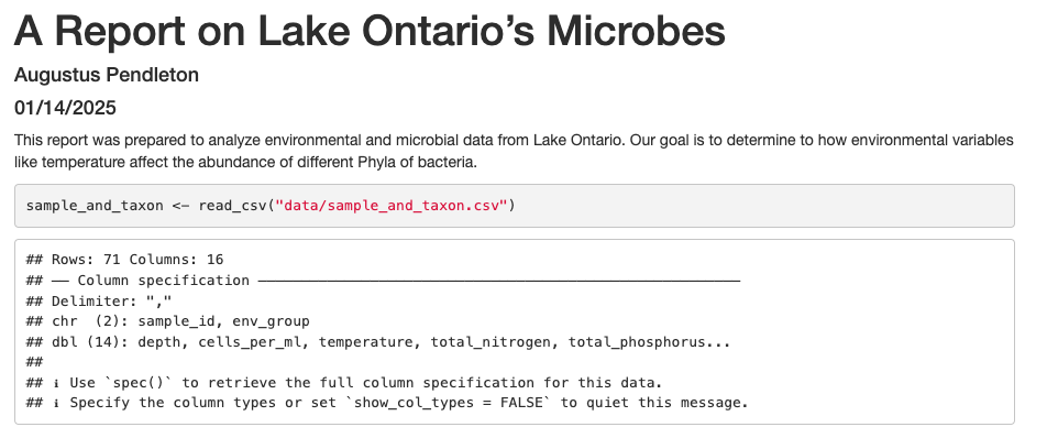
To get rid of this, we can revise our packages code chunk by adding include=FALSE just like in the setup chunk to prevent code and messages in this chunk from showing up in our report.
```{r packages, include=FALSE}
library(tidyverse)
```
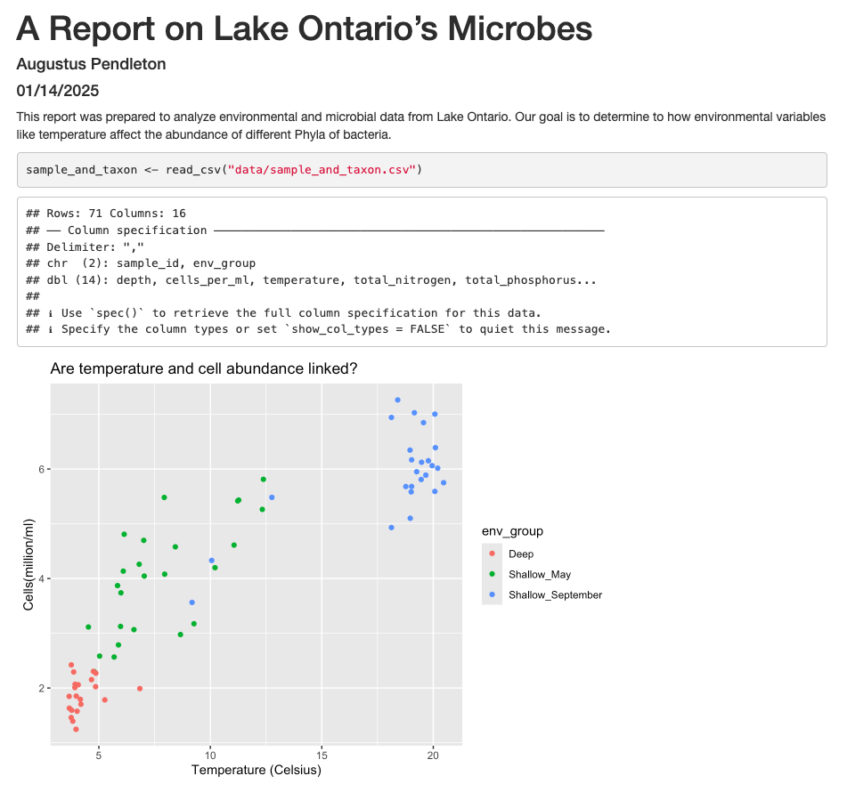
We can also see the code that was used to generate the plot. Depending on the purpose and audience for your report, you may want to include the code. If you don’t want the code to appear, how can you prevent it? What happens if we add include=FALSE to the plot code chunk, too? Try rendering the R Markdown report with this change.
Oops! Now the plot doesn’t show up in our report at all. This is because setting include=FALSE prevents anything in the code chunk from appearing in the report. Instead we can add echo=FALSE to tell this code chunk that we don’t want to see the code but just the output.
```{r cell_vs_temp, echo = FALSE}
ggplot(data = sample_and_taxon) +
  aes(x = temperature, y = cells_per_ml/1000000, color=env_group) +
  geom_point() +
  labs(x = "Temperature (Celsius)", y = "Cells(million/ml)",
       title= "Are temperature and cell abundance linked?")
```
When we knit this again, our plot is back!
Before we finalize our report, let’s look at a few other cool features. Sometimes, you want to describe your data or results (like our plot) to the audience in text but the data and results may still change as you work things out. R Markdown offers an easy way to do this dynamically, so that the text updates as your data or results change. Here is how to do this.
First, let’s create a code chunk that summarizes features of our data that we can use to describe our plot to our audience. Note that we set include=FALSE because we only want this step to happen in the background. For our purposes, we will calculate how many samples were included in the analysis, as well as the minimum and maximum temperature values:
```{r data_summary, include=FALSE}
nSamples <- sample_and_taxon %>%
  select(sample_id) %>%
  n_distinct()

minTemp <- sample_and_taxon %>%
  summarise(round(min(temperature))) %>%
  pull()

maxTemp <- sample_and_taxon %>%
  summarise(round(max(temperature))) %>%
  pull()
```
Now, all we need to do is reference the values we just computed to describe our
plot. To do this, we enclose each value in one set of backticks
(`r some_R_variable_name `), while the r part once again
indicates that it’s a chunk of R code. When we knit our report, R will
automatically fill in the values we just created in the above code chunk. Note
that R will automatically update these values every time our data might change
(if we were to decide to drop or add samples to this analysis, for example).
The above plot shows the relationship between cell abundance and temperature for a total of `r nSamples ` samples. For this set of samples, temperature ranged from a minimum of `r minTemp`°C
to a maximum `r maxTemp`°C.
Formatting
We now know how to create a report with R Markdown. Maybe we also want to format the report a little bit to structure our thought process in a useful way (e.g., sections) and make it visually appealing? Markdown is a very simple programming language when it comes to syntax. Let’s try to figure out some syntax together. Suppose we wanted to create sections in our report.
R Markdown headers
Try googling how to create sections by using headers and subheaders using R Markdown. What do you find?
Solution
We can easily create headers and subheaders by using the
#pound/hash sign. Our main headers have one#(e.g.# Main Header Here) and to create subheaders we add additinal#s (e.g.## First subheaderand### Second subheader)
OK, now that we know how to make headers, let’s practice some more Markdown syntax.
R Markdown syntax
Go ahead and do some online searches on how to do the following:
- create a bullet point list with three items
- as the first item, write the name of your currently favorite programming language in bold
- as the second item, write the name of a function you have so far found most useful in italics
- as the third item, write one thing you want to learn next on your programming journey in bold and italics
- turn your bullet point list into a numbered list
- create a fourth list item and find an online guide and/or cheat sheet for basic Markdown syntax, write its name down here and hyperlink its url
Solution
This link has some helpful basic R Markdown syntax.
- To create bullet points, use
-or*on each line- To make something bold, wrap the words in two asterisks:
**- To make something italic, wrap the words in one asterisk:
*- To make something bold and italic, wrap the words in three asterisks:
***- To make a numbered list, use
1.,2., etc. on each line- To make a hyperlink, wrap the words in square brackets followed by the url in parentheses
[sentence to link](url)
Using the “Visual” view for easy formatting
In newer versions of RStudio, we can switch to the “Visual” view when editing our documents. This makes the experience much more similar to writing in software like Microsoft Word or Google Docs. We can use formatting tools (like bolding and italicizing), insert pictures, and create tables without manually typing out the markdown syntax. The best part? If you then switch back to the “Source” view, you can see the markdown syntax RStudio has automatically created for you.
Knitting to PDF
So far, we’ve been knitting our documents to produce an HTML document. HTML is the language used by web developers to make websites - browsers like Chrome or Safari read HTML and display it to you as a beautiful site. HTML documents have many benefits: they tend to be flexible which is nice for large figures, long lines of code, or large tables and you can easily change the theme. It’s also easy to quickly use HTML documents to produce websites which you can send to people or link via QR codes. However, sometimes we want PDF documents, which are easy to print or share via email.
By installing the package knitr, we were able to knit our Rmarkdown documents to HTML. To knit to PDF, we need to install an additional software packages. We’ll first install the R package tinytex. This R package will then help us install a different software, called TinyTeX (pronounced “Tiny-TECK”), which can translate our RMarkdown document to a PDF.
In the console, type:
install.packages("tinytex")
This will install the R package tinytex. Next, we’ll use a function within the tinytex package to install the TinyTeX software
tinytex::install_tinytex()
Finally, we’re going to change our YAML header to reflect that we should knit to PDF.
---
title: 'Writing Reports with R Markdown'
author: "Augustus Pendleton"
date: "01/14/2025"
output: pdf_document
---
Now, let’s click the “Knit” button. We should see our new PDF document rendered!
Key Points
R Markdown is an easy way to create a report that integrates text, code, and figures.
Options such as
includeandechodetermine what parts of an R code chunk are included in the R Markdown report.R Markdown can render HTML, PDF, and Microsoft Word outputs.